The Conversation (1)

Time and Tide: This mechanical analog computer was used for predicting tides. Known as “Old Brass Brains” (or more formally, Tide-Predicting Machine No. 2), it served the U.S. Coast and Geodetic Survey in the calculation of tide tables beginning in 1912 and was not retired until 1965, when it was replaced with an electronic computer.
Illustration/Photo: NAOO
When Neil Armstrong and Buzz Aldrin landed on the moon in 1969 as part of the Apollo 11 mission, it was perhaps the greatest achievement in the history of engineering. Many people don’t realize, though, that an important ingredient in the success of the Apollo missions and their predecessors were analog and hybrid (analog-digital) computers, which NASA used for simulations and in some cases even flight control. Indeed, many people today have never even heard of analog computers, believing that a computer is, by definition, a digital device.
If analog and hybrid computers were so valuable half a century ago, why did they disappear, leaving almost no trace? The reasons had to do with the limitations of 1970s technology: Essentially, they were too hard to design, build, operate, and maintain. But analog computers and digital-analog hybrids built with today’s technology wouldn’t suffer the same shortcomings, which is why significant work is now going on in analog computing in the context of machine learning, machine intelligence, and biomimetic circuits.
Here, I will focus on a different application of analog and hybrid computers: efficient scientific computation. I believe that modern analog computers can complement their digital counterparts in solving equations relevant to biology, fluid dynamics, weather prediction, quantum chemistry, plasma physics, and many other scientific fields. Here’s how these unconventional computers could do that.
An analog computer is a physical system configured so that it is governed by equations identical to the ones you want to solve. You impose initial conditions corresponding to those in the system you want to investigate and then allow the variables in the analog computer to evolve with time. This result provides the solution to the relevant equations.
Most early analog computers were mechanical contraptions containing rotating wheels and gears
To take a ludicrously simple example, you could consider a hose and a bucket as an analog computer, one that performs the integration function of calculus. Adjust the rate of water flowing in the hose to match the function you want to integrate. Direct the flow into the bucket. The solution to the mathematical problem at hand is just the amount of water in the bucket.
Although some actually did use flowing fluids, most early analog computers were mechanical contraptions containing rotating wheels and gears. These include Vannevar Bush’s differential analyzer in 1931, constructed on principles that go back to the 19th century, chiefly to the work of William Thomson (who later became Lord Kelvin) and his brother James, who designed mechanical analog computers for calculating tides. Analog computers of this sort remained in use for a long time for such purposes as controlling the big guns on battleships. By the 1940s, electronic analog computers took off too, although the mechanical variety continued in use for some time. And none other than Claude Shannon, the father of formal digital design theory, published a seminal theoretical treatment of analog computing in 1941.
Starting at about that time, electronic analog computers were extensively developed in the United States, the Soviet Union, Germany, the United Kingdom, Japan, and elsewhere. Many manufacturers, including Electronic Associates Inc., Applied Dynamics, RCA, Solartron, Telefunken, and Boeing, produced them. They initially were used in missile and airplane design and in-flight simulators. Naturally enough, NASA was a major customer. But applications soon extended to other areas, including nuclear-reactor control.
aspect_ratio Plug and Play: This electronic analog computer, the PACE 16-31R, manufactured by Electronic Associates Inc., was installed at NASA’s Lewis Flight Propulsion Laboratory (now called the Glenn Research Center), in Cleveland, in the mid-1950s. Such analog computers were used, among other things, for NASA’s Mercury, Gemini, and Apollo programs.Photo: NASA
Electronic analog computers initially contained hundreds or thousands of vacuum tubes, later replaced by transistors. At first, their programming was done by manually wiring connections between the various components though a patch panel. They were complex, quirky machines, requiring specially trained personnel to understand and run them—a fact that played a role in their demise.
Another factor in their downfall was that by the 1960s digital computers were making large strides, thanks to their many advantages: straightforward programmability, algorithmic operation, ease of storage, high precision, and an ability to handle problems of any size, given enough time. The performance of digital computers improved rapidly over that decade and the one that followed, with the development of MOS (metal-oxide-semiconductor) integrated-circuit technology, which made it possible to place on a single chip large numbers of transistors operating as digital switches.
Analog-computer manufacturers soon incorporated digital circuits into their systems, giving birth to hybrid computers. But it was too late: The analog part of those machines could not be integrated on a large scale using the design and fabrication techniques of the time. The last large hybrid computers were produced in the 1970s. The world moved to digital computers and never looked back.
Today analog MOS technology is highly advanced: It can be found in the receiver and transmitter circuits of smartphones, in sophisticated biomedical devices, in all manner of consumer electronics, and in the many smart devices that make up the Internet of Things. If constructed using this highly developed, modern technology, analog and hybrid computers could be very different animals from those of half a century ago.
But why even consider using analog electronics to do computation? Because conventional digital computers, powerful as they are, may be reaching their limits. Each time a digital circuit switches, it consumes energy. And the billions of transistors on a chip switching at gigahertz speeds produce a lot of heat, which somehow must be removed before it causes damaging temperatures to build up. It’s easy to find clips on YouTube demonstrating how to fry an egg on some of today’s digital computer chips.
Energy efficiency is of particular concern for scientific computation. That’s because the flow of time in a digital computer must be approximated as a series of discrete steps. And in solving certain challenging kinds of differential equations, extremely fine time steps are needed to ensure that the algorithm involved comes to a solution. This means that a very large number of calculations is needed, which takes a long time and consumes a lot of energy.
About 15 years ago, I began to wonder: Would an analog computer implemented with today’s technology have something valuable to offer? To help answer that question, Glenn Cowan—a doctoral student I was then advising at Columbia and now a professor at Concordia University in Montreal—designed and built an analog computer on a single chip. It contained analog integrators, multipliers, function generators, and other circuit blocks, laid out in the style of a field-programmable gate array. That is, the various blocks were embedded in a sea of wires that could be configured to form connections after the chip was fabricated.
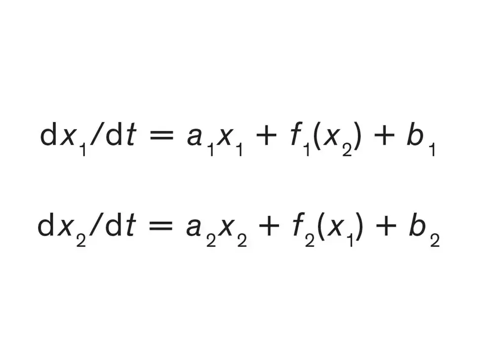
Many scientific problems involve solving systems of coupled differential equations. For simplicity here, we consider two differential equations governing two variables, and x2. An analog computer solves for x1 and x2 using a circuit in which the currents flowing in two wires are governed by the very same equations. With the appropriate circuit, the currents in those two wires will swiftly represent the solution to the original equations.

Digital programming made it possible to connect the input of a given analog block to the output of another one, creating a system governed by the equation that had to be solved. No clock was used: Voltages and currents evolved continuously rather than in discrete time steps. This computer could solve complex differential equations of one independent variable with an accuracy that was within a few percent of the correct solution.
For some applications, this limited accuracy was good enough. In cases where it was too crude, we could feed the approximate output to a digital computer for refinement. Because the digital computer was starting with a very good initial guess, speedups of a factor of 10 or so were easily achievable, with energy savings of similar magnitude.
More recently at Columbia, two students, Ning Guo and Yipeng Huang; two of my faculty colleagues, Mingoo Seok and Simha Sethumadhavan; and I created a second-generation single-chip analog computer. As was the case with early analog computers, all blocks in our device operated at the same time, processing signals in a way that in the digital realm would require a highly parallel architecture. And we now have larger chips composed of several replicas of our second-generation design, which can solve problems of greater size.
The new design for our analog computer is more efficient in its use of power and can more easily connect with digital computers. This hybrid form of computing provides the best of both worlds: analog for approximate computations achieved with high speed using little energy, and digital for programming, storage, and computation with high precision.
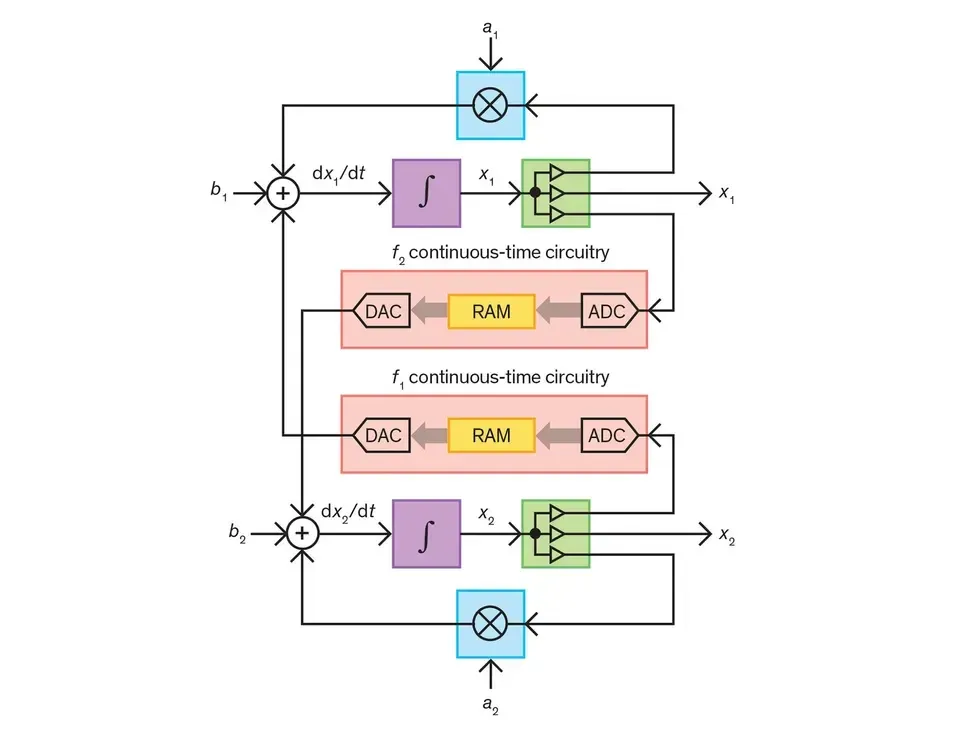
Our latest chip contains many circuits that have been used in the past for analog computation: ones that integrate or multiply, for example. But a key component in our new design is a novel circuit that can continuously compute arbitrary mathematical functions. Here’s why it’s important.
Digital computers operate on signals that assume just two voltage levels, representing the values of 0 and 1. Of course, when shifting between those two states, the signals must take on intermediate voltages. But typical digital circuits process their signals only periodically, after the signal voltages have stabilized at values that clearly represent 0 or 1. These circuits do so by means of a system clock, which has a period that is long enough for voltages to switch from one stable level to another before the next round of processing occurs. As a result, such a circuit outputs a sequence of binary values, one with each tick of its clock.
Our function generator is based instead on an approach my colleagues and I developed, which we call continuous-time digital. It involves clockless binary signals that can change value at any instant, rather than at pre-defined times. We’ve built analog-to-digital and digital-to-analog converters, as well as a digital memory, that can handle such continuous-time digital signals.
We can feed an analog signal into such an analog-to-digital converter, which translates it to a binary number. That number is used to look up a value stored in memory. The output value is then fed into a digital-to-analog converter. The combination of these continuous-time circuits gives a programmable analog-in, analog-out function generator.
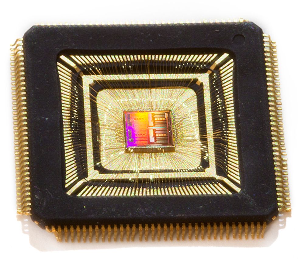 Cool and Calculating: The author and his colleagues used modern fabrication technology to pack a powerful analog computer into a tiny package.Photo: Randi Klett
We have used our computer to solve some challenging kinds of differential equations to an accuracy of a few percent. That’s pretty poor in comparison with what’s normally achievable on a digital computer. But accuracy isn’t everything. Indeed, in many cases, working with approximate values is good enough. Approximate computing—purposefully limiting the accuracy of the calculations—is sometimes used in today’s digital computers, for example in such fields as machine learning, computer vision, bioinformatics, and big-data mining. It makes sense when the inputs themselves are approximate, as is often the case.
Because the core of our computer is analog, it can interface directly with sensors and actuators if need be. And its high speed allows for real-time interactions with the user in computational tasks that otherwise would be impossibly slow.
Of course, our approach to computing still has some rough edges. One challenge is that particularly complicated problems require lots of analog computational blocks, making for a large and therefore expensive chip.
One way to address this issue is to divide the computational problem at hand into smaller subproblems, each solved in turn by an analog computer working under the supervision of a digital computer. The computation would no longer be completely parallel, but at least it would be possible. Researchers explored this approach decades ago, when hybrid computers were still in vogue. They didn’t get far before such computers were abandoned. So this technique will require further development.
Another issue is that it is difficult to configure arbitrary connections between distant circuit blocks in a large analog-computing chip: The wiring net needed for that would become prohibitive in size and complexity. Yet some scientific problems would require such connections if they are to be solved on an analog computer.
Three-dimensional fabrication technologies may be able to address this limitation. But for now, the analog core of our hybrid design is best suited to applications where local connectivity is all that is needed—for example, the simulation of arrays of molecules that interact with nearby molecules but not with those far away.
Because the core of our computer is analog, it can interface directly with sensors and actuators if need be
Yet another hurdle is the difficulty implementing multivalued functions and the related problem of handling partial differential equations efficiently. Several techniques for solving such equations with hybrid computers were under development in the 1970s, and we intend to pick up where earlier researchers left off.
Analog also has a disadvantage when it comes to increasing precision. In a digital circuit, precision can be increased just by adding bits. But increasing precision in an analog computer requires the use of significantly larger chip area. This is why we have targeted low-precision applications.
I’ve said that analog computing can speed calculations and save energy, but I should be more specific. The analog processing on a computer of the type my colleagues and I have developed typically takes about a millisecond. The solution of differential equations that involve only one derivative typically requires less than 0.1 microjoules of energy on our computer. And it takes one half of a square millimeter of chip area if we use plain-vanilla fabrication technology (65-nm CMOS). Equations that involve two derivatives take twice as much energy and area, and so forth; yet the solution time remains the same.
For certain critical applications for which cost is no object, we might even consider wafer-scale integration—the entire silicon wafer could be used as a huge chip. With a 300-millimeter wafer, this would permit more than 100,000 integrators to be placed on the chip, thus allowing it to simulate a system of 100,000 coupled first-order nonlinear dynamical equations, or 50,000 second-order ones, and so forth. This might be useful, for example, in simulating the dynamics of a large array of molecules. The solution time would still be in the milliseconds, and the power dissipation in the tens of watts.
Only experiments can confirm that a computer of this type would actually be feasible and that the accumulation of analog errors would not conspire against it. But if it did work, the result would be far beyond what today’s digital computers can do. For them, some of the more difficult problems of this size require an immense amount of power or solution times that can stretch into days or even weeks.
Clearly, much investigation remains to be done to sort out the answers to this and other questions, such as: how to distribute the tasks between the analog and digital parts, how to break a large problem down to smaller ones, and how to combine the resulting solutions.
In pursuing those answers, we and other researchers newly interested in analog computers can benefit from the work done by many very smart engineers and mathematicians half a century ago. We shouldn’t try to reinvent the wheel. Rather, we should use earlier results as a springboard and go much further. At least, this is our hope, and we will never know for sure until we try.
Editor’s Note: Following publication of this article, the author learned that the concept of the function generator mentioned in it was described earlier in U.S. Patent No. 5,006,850, by Gordon J. Murphy. The author would like to thank Professor Murphy for bringing this patent to his attention.
About the Author
Yannis Tsividis is the Edwin Howard Armstrong Professor of Electrical Engineering at Columbia University.


