Not all power plants are the same. They certainly don’t cost the same to build or operate. But what if I told you that one number, dubbed the levelized cost of electricity (LCOE), puts it all into black and white for decision makers: This plant’s electricity is cheaper than that one’s, or it isn’t.
LCOE is the estimated amount of money that it takes for a particular power plant to produce a kilowatt-hour of electricity over its expected lifetime and is typically expressed as cents per kilowatt-hour or dollars per megawatt-hour.
LCOE makes it easy to decide which plant to build if you’re a utility or a governing agency. Except that LCOE misses a few important location-based factors, such as fuel delivery costs, construction costs, capacity factors, utility rates, financing terms, and other geographically distinct items that contribute to the cost of a kilowatt-hour.
Despite these shortcomings, LCOE has become the de facto standard for cost comparisons among the general public, policymakers, analysts, advocacy groups, and other stakeholders. One number is readily understood, easily bandied about, and even more easily compared to any other number.
To address LCOE’s lack of geographical considerations, my team, via The Full Cost of Electricity (FCe-) study coordinated by the Energy Institute at the University of Texas at Austin, developed and applied a geographically resolved method to calculate the LCOE of new power plants on a county-by-county basis—while including estimates of some environmental externalities.
We calculated the LCOE for each county of the contiguous United States for 12 power plant technologies: two types of coal, each with partial and full carbon capture and sequestration (CCS); natural gas combined cycle with and without CCS; natural gas combustion turbine; nuclear; onshore wind; solar photovoltaic (PV), both utility-scale and residential; and concentrating solar power with 6 hours of storage.
The lowest LCOE option for each county varies based on local conditions, capital and fuel costs, environmental externalities, and resource availability. While the average cost increases—when internalizing the environmental externalities of such particulates and pollutants as SO2, NOx, PM10, PM2.5, CO2, and CH4—are small for some technologies, the local cost differences can be as high as US $0.62 per kilowatt-hour for some generation types. This holds true when not including the externalities also.
People like to discuss our input assumptions and play with their own, so we developed interactive online tools: Two interactive calculators are available to estimate LCOE per county and technology to facilitate policy-level discussions about the costs of different electricity options. Enter your own numbers and make your own maps here:
Methods and reasonable (in our estimation) starting points for capital and operating expenses, fuel prices, capacity factors, and all the other aspects that go into LCOE calculations can be found in our white paper, “A Geographically Resolved Method to Estimate Levelized Power Plant Costs with Environmental Externalities,” and as defaults in our online interactive calculators. (IEEE Spectrum is posting blogs from the UT researchers and linking to the white papers as they are released.)
Maps of results facilitate comparisons by fuel, technology, and location. They offer the ease of the single number but put more information behind it.
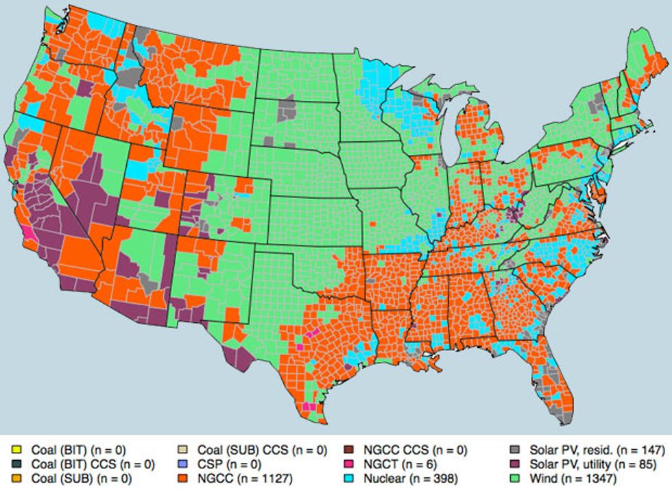
The map shows the minimum cost technology for each county in a scenario where we consider externalities and availability zones. In locations where the wind resource is strong and/or barriers (nonattainment zones or water availability, for example) are high for thermal plants, wind tends to be the lowest-cost option.
Using our method, we found that:
- Wind (green) is the lowest cost option in most counties.
- Natural gas combined cycle (NGCC, red-orange) is the least-cost option in counties where the wind resource isn’t as strong.
- Nuclear plants (blue) are the least-cost technology where wind resources are marginal and gas prices are high or natural gas pipelines are not available.
- Residential solar PV (gray) plants are the default option when a county was otherwise excluded by one or more barriers to other technologies.
- Utility-scale solar PV (purple) plants are clustered in locations that have excellent solar insolation levels and/or lack of cooling water availability.
- Natural gas combustion turbine plants (pink) are located where conditions are also favorable to NGCC plants but lack cooling water availability.
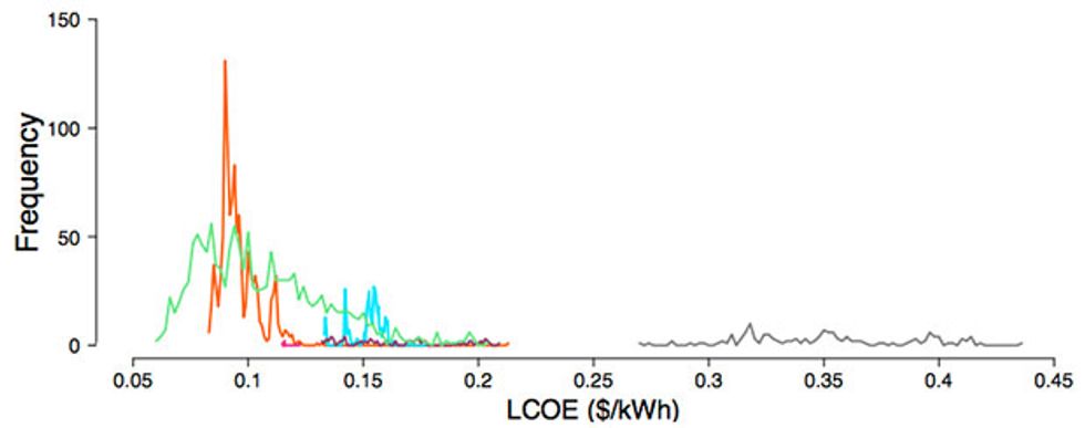
The average reference case cost for all the counties’ minimum cost technologies was $0.127/kWh (median: $0.102/kWh). The lowest county-specific LCOE is near $0.06/kWh (from wind power) and the highest (not including residential PV) is approximately $0.21/kWh. When externalities are included using our default assumptions, neither coal, nor any carbon capture and sequestration technology, nor concentrating solar power (CSP) is the cheapest technology in any location.
This analysis considers the cost to produce electricity, not what the electricity price is in a given region. That is to say, we are discussing costs, not revenues and profits. Market prices for power change throughout the day. Our LCOE analysis does not take seasonal or diurnal price variation into consideration. While relevant for estimating profitability of all technologies, and particularly relevant for intermittent generation technologies (solar, for example, usually produces a greater share of its total generation during times of higher electricity prices than wind), the consideration of seasonal and daily prices is beyond the scope of LCOE. However, this might also change as more and more renewables come on line as referenced by California’s Duck Curve [PDF].
Joshua Rhodes is a postdoctoral research fellow at the University of Texas at Austin Energy Institute.